All Blogs
What is PI?
To put it simply, PI is the ratio of a circles circumference to its diameter. We can find the irrational constant with the following calculation. Assuming we have a circle with a diameter $D$, we then measure the circumference $C$ of the circle. $\pi$ can then be calculated by $C/D$.
$$ \begin{aligned} let \quad D &= 5, \\ C &= 15.72 \\ \therefore \quad \pi &\approx \frac{C}{D} = \frac{15.72}{5} = 3.144 \end{aligned} $$
Its not particularly accurate, but neither was the measurement I got for the circumference. Now we know how to calculate PI by 2 measurable quantities, it doesn't take much to see why the circumference of a circle is found by the formula $C = 2 \pi r = \pi D$. So if we had a circle with a diameter of 1, it's circumference would be equal to $\pi$.
As a side note, we can find the equation for the area of a circle by integrating the circumference equation (integration gives the area under a curve).
$$ \begin{aligned} C &= \pi D = 2\pi r\\ A &= \int 2\pi r \, dr = \pi r^2 \end{aligned} $$
Approximating PI
While the above method will give us a value for $\pi$, it's not exactly easy/possible to calculate via a computer, i.e., how do you measure the circumference of a circle draw on a screen automatically? The answer is... you don't. There are many other ways of calculating the decimal places of $\pi$. The Gauss-Legendre algorithm is a particularly interesting example of how to calculate $\pi$ (more can be found here). It's an iterative algorithm, whereby each pass through doubles the precision for the value of $\pi$. Since I write code in Erlang for a living, I have also provided an example solution for the algorithm here. It is worth noting, that running the algorithm past 3 iterations will just return the same number. This is because of the limit to floating point numbers in Erlang.
Monty Carlo Method
For this post however, I am going to use a pretty basic Monty Carlo method. The idea is to place a unit circle inside a 1x1 square. We can then get a formula for $\pi$ based off the ratio of the circle's area and the square's area. $A_c$ is the area of the circle, $A_s$ is the area of the square.
$$ \begin{aligned} A_c &= \pi r^2 \\ A_s &= (2r)^2 = 4r^2 \\ \frac{A_c}{A_s} &= \frac{\pi r^2}{4r^2} = \frac{\pi}{4} \end{aligned} $$
Given the above, we can see that $\pi$ can be calculated as $4 \times \frac{A_c}{A_s}$. The simulation below uses random sampling to produce a value for this ratio thus letting us approximate $\pi$ (albeit very badly).
0
1000
$\pi \approx$ 4 * Inside / All
Accuracy = | Math.PI - PI Approximation |
Links:
Gauss-Legendre algorithm | Other algorithms | Monty Carlo Pi Approximation | Gauss-Legendre (Erlang Implentation)
What is Docker
Docker is a CI/CD tool that utilises containers for code deployment. Docker containers are instantiated from a composition of many docker images. Ranging from a simple OS level image to more advanced automatic build and deployment images. Docker images are generated from simple Dockerfiles which lay out the commands that the container runs either before or after its instantiation. Docker is useful when wanting to run the same piece of code on different machine architectures as it works much like a virtual machine would.
CLI tools
This section describes some of the command line tools that docker offers, as well as some useful tricks.
Login
Generally the first thing that you should do when running docker is to login. This is done with the
docker login
command. You will then be prompted for your docker username and password.
Running a container
Once logged in, the next step is to run an image. This is done via the
docker run imagename
command. If the image is not currently downloaded to your computer then it will be downloaded from the docker hub. You can update a previously downloaded image by using the
docker pull imagename
command. The
run
command is often run with several flags. A particularly useful flag is the
--name
flag, which lets you set a name for the container that you can use in other commands later on.
-p port:externalport
can map an exposed port in the container to a system port, i.e., running several of the same container and mapping different ports to the containers without having to change the code.
-d
lets you run the container as a background process.
Container management
Much like in a linux terminal, you can use
ps
to show the currently running containers. The flag
-a
shows all of the containers on the system.
You can remove a container with the
docker rm container
. If the container is currently running, you can either stop it with
docker stop
or use the
-f
flag to forcefully remove the container. You can remove all of the containers on the machine indescriminately by running the following
docker rm $(docker ps -a -q)
. Alternatively you can use the
--rm
flag when running the image so that the container is removed when it exits.
Images
To see a list of the currently downloaded images on the computer run the
docker images
command. To remove a specific image you can use the
docker rmi imagename
command.
Arguably the most important part of docker is the ability to create your own images with ease. This is done by using a dockerfile and then calling the
build
command. The easiest way of doing this is inside the same directory that the dockerfile is in. It is important to give the image a tag so that it can be easily referred to later on.
docker build -t imagename .
.
Once the image has been built, you can link it to a remote repo in the docker hub by using the
docker tag localname remote/name
. The once a link has been made, push the image to the hub
docker push remote/name
.
Dockerfiles
Dockerfiles are what docker uses to build the docker images. Each docker file contains a base docker image defined by the
FROM image
statement. This image is then built upon by using various other rules. The most common other rules being
RUN
and
ADD
.
RUN
will execute a system command for the OS defined by the base image.
ADD
will copy files from the build computer to the container.
Below is an example of how to create a golang dockerfile via a ubuntu image.
FROM ubuntu

MAINTAINER Mark Hillman

# Add the go path to the system
ENV GOPATH /go

# Copy over the files to the gopath dir
ADD . /go/src/github.com/imitablerabbit/go-project

# Update and install golang via apt
RUN apt-get update && \
	apt-get install -y golang && \
	go install github.com/imitablerabbit/go-project

# Set the entrypoint of the container.
ENTRYPOINT /go/bin/go-project

# Expose the port
EXPOSE 8080
There is a much better way though. You can just use the pre-existing golang images. The following example is based on the Go blog docker examples.
FROM golang:1.6-onbuild
MAINTAINER Mark Hillman
EXPOSE 80
Links:
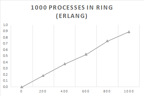
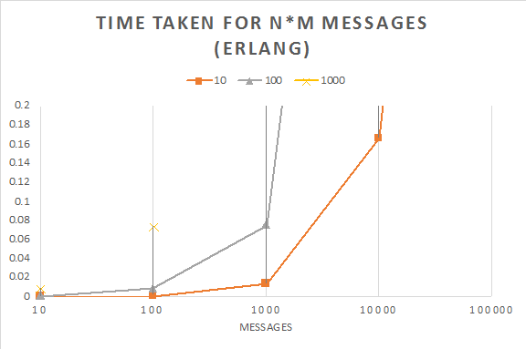
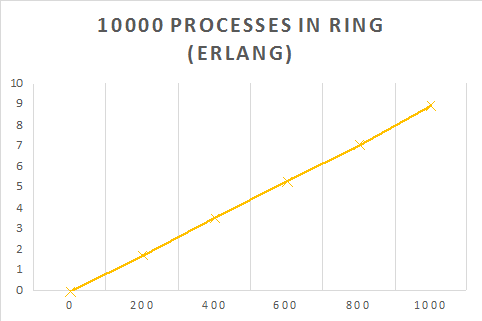
This post is about exercise 3 in chapter 12 of the Programming Erlang - Software for a Concurrent World book. The premise of the exercise is to create a ring of concurrent processes which each send a message around the ring. The message should be passed $M$ times around a ring of $N$ processes. The completion time is then measured for the $M \cdot N$ messages passed and plotted on graphs to compare complexity and efficiency between the languages.
So, for the exercise I decided that Go would be a suitable competitor to Erlang as they can both create processes/goroutines easily and cheaply. Unfortunately, as I am more experienced with Go, the results might be in favour for Go. In order to try and mitigate any discrepancies, I am going to try and create very similar ways of passing the message around the ring.
Erlang Ring
For the Erlang ring, as I am not sure how to create structures (If you can at all) the best thing I could do is to spawn all the processes and store their Pid's in a list. When first creating the ring, I would access the required ring element by using the lists:nth function along with an index passed along in the message. This was soon changed to having a spent ring process list and the upcoming process list. Then when one process in the ring has been sent a message, it is moved to the spent list. This increased the performance of the ring operations significantly as it is $O(1)$ rather than $O(n).$ In the most recent version of the code, the ring has been constructed so that each process controls the Pid for the next process in the ring by passing it to the ring_element function. With the new changes in the erlang code, the differences between the code are minimal and so should be a more accurate test. The code for the erlang ring looks somewhat like the following.
% create_ring will return the data structure which is used
% for all of the ring functions. This is essentially a list of
% Pid's for processes which have already been spawned and are
% waiting for a message from the previous process in the ring.
%
% N - the number of processes in the ring
%
create_ring(N) ->
Pid = spawn(ring, ring_start, []),
create_ring(N, [Pid], Pid).
create_ring(1, [PPid|Acc], Start) ->
Start ! {PPid},
Ring = [PPid|Acc],
lists:reverse(Ring);
create_ring(N, [PPid|Acc], Start) ->
Pid = spawn(ring, ring_element, [PPid]),
NewAcc = [Pid|[PPid|Acc]],
create_ring(N-1, NewAcc, Start).
% ring_element will handle the passing of a message to the
% next process in the ring. This happens until the message
% reaches the end of the ring.
%
% NPid - this is the Pid of the next ring member
%
ring_element(NPid) ->
receive
Payload ->
NPid ! Payload,
ring_element(NPid)
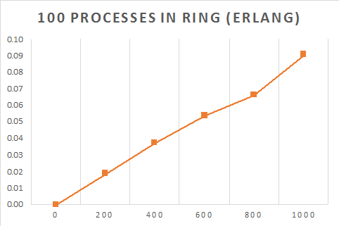
end.The table below shows the time taken (s) for a message to be sent $M$ times around a ring of $N$ processes.
| Processes | Number of times message sent around the ring ($M$) | |||||
|---|---|---|---|---|---|---|
| 0 | 200 | 400 | 600 | 800 | 1000 | |
| 100 | 0 | 0.019014 | 0.037506 | 0.054008 | 0.066509 | 0.09101 |
| 1000 | 0 | 0.188024 | 0.376047 | 0.529625 | 0.744093 | 0.893612 |
| 10000 | 0 | 1.755221 | 3.562469 | 5.322169 | 7.069391 | 8.983079 |
Go Ring
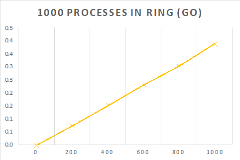
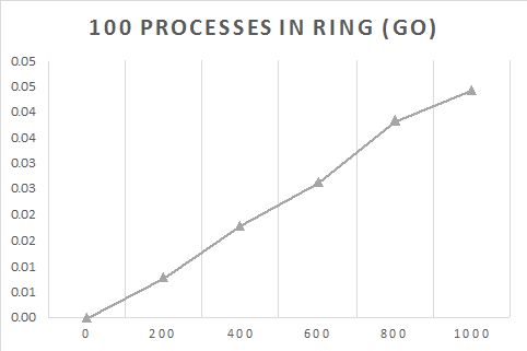
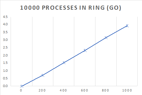
The Go ring is fairly similar to the Erlang ring except that it uses structures to hold the next Node as a pointer. The communication between the nodes is via a channel, which is the closest method to Erlang's send primitive. However, the Go code has been optimised somewhat in that only the start of the ring has to check when the message has gone around the ring, which saves a lot of computation. Thus the Go code will be a fair bit faster. The most important part of this blog is to just show the linear relation between creating more processes and the time taken to complete the message sending. The following is a snippet of the Go code.
// StartNodes takes a ring of nodes and starts the processes. It also
// creates a channel for the ring to send back information on when it
// is completed. This function will block until the ring has finished
func (r *Ring) StartNodes() {
	reply := make(chan bool)
	go r.Start.HandleStartNode(r.MessageNum, reply)
	for current := r.Start.Next; current != r.Start; current = current.Next {
		go current.HandleNode()
	}
	r.Start.In <- r.Message
	<-reply
}

// HandleNode will receive and send any messages in the ring
// this is how the ring works. When the ring should no longer send
// a message the channel is closed.
func (n *Node) HandleNode() {
	for message := range n.In {
		n.Next.In <- message
	}
}| Processes | Time taken for $M$ processes (s) | |||||
|---|---|---|---|---|---|---|
| 0 | 200 | 400 | 600 | 800 | 1000 | |
| 100 | 0 | 0.0080012 | 0.018002 | 0.0265028 | 0.0385034 | 0.0445047 |
| 1000 | 0 | 0.0760249 | 0.1530192 | 0.2320464 | 0.3050381 | 0.389548 |
| 10000 | 0 | 0.7300922 | 1.528035 | 2.3277921 | 3.1648963 | 3.9280171 |
Screenshots:
Links:
Manipulation of Sums
As the book covers the distributive and associative laws very well, this section will only focus on the commutative law. The book states that the sum of integers in the finite set $K$ can be transformed with a permutation $p(k).$ The law looks as follows
$$ \sum \limits_{k \in K} a_k = \sum \limits_{p(k) \in K} a_{p(k)}. $$
Put simply, this means that the sum remains the same as long as all the elements in the set get summed, just in a different permutation. A simple example of this is $p(k) = -k$, which is the same set just in reverse. The book gives an example of the set $K = \{ -1, 0, 1 \}$, so the permutation $p(k) = -k$ gives
$$ a_{-1} + a_0 + a_1 = a_1 + a_0 + a_{-1} $$
While this example isn't too taxing, the following is a little harder to understand. This next example is how Gauss's trick from Chapter 1 can be found using the different manipulation laws. The first step in the example is the most confusing as it is the one which features the commutative law. We start with
$$ S = \sum \limits_{0 \le k \le n}(a + bk). $$
The book says that we now replace $k$ with $n - k.$ Sadly it does little to explain why this is the case. Well, we can show the permutation more clearly by creating a new variable called $k_1$ and saying $k_1 = n - k$, which we can rearrange for $k$ and plug it back into the sum.
$$ \sum \limits_{0 \le k \le n}(a + bk) = \sum \limits_{0 \le n - k_1 \le n}(a + b(n - k_1)) $$
Now it pays to look at the bounds of the sum, $0 \le n - k_1 \le n$ is technically the same as $0 \le k_1 \le n$ (We know this to be true as $n - k_1$ is just the reverse of $k_1$). So we can substitute this back into the summation.
$$ S = \sum \limits_{0 \le k_1 \le n}(a + b(n - k_1)) $$
Now as $k_1$ is just a simple variable, we can replace its letter with $k$. This gives us
$$ S = \sum \limits_{0 \le k \le n}(a + b(n - k)) $$
Just to prove that these are the same, we can expand out the sum to show the individual components for each summation.
$$ \begin{aligned} \sum \limits_{0 \le k \le n}(a + bk) &= (a + b \cdot 0) + (a + b \cdot 1) + \ldots + (a + b \cdot n) \\ \sum \limits_{0 \le k \le n}(a + b(n - k)) &= (a + b \cdot (n - 0)) + (a + b \cdot (n - 1)) + \ldots + (a + b \cdot (n - n)) \end{aligned} $$
You can see that these are essentially the same just with the later summing down. The book now walks us through the other laws with the same example, but those are not too hard to understand, so I won't be covering them here.
Links with Integration
The book suggests we can use the concept of integrals to solve sums. This is first introduced by showing an example in method 4 of chapter 2.5. Unfortunately, it doesn't quite work out as it leaves a small error term. Fortunately, the book's next section shows the real connection between integration and summation.
It is worth noting that the book uses different notation than some people might be used to, e.g $D(f(x)) = \frac{d}{dx} f(x).$ The equation for a derivative that the book uses is more commonly known as
$$ \frac{d}{dx} f(x) = \lim_{\Delta x \to 0} \frac{f(x + \Delta x) - f(x)}{\Delta x}. $$
Now the book introduces finite calculus. This is the same as infinite calculus (integration/differentiation) but restricted to integers. This means that $\Delta x = 1$ is the lowest value we can get to with a limit approaching 0 using integers. Therefore the derivative for finite calculus is
$$ \Delta f(x) = f(x + 1) - f(x). $$
This isn't super useful yet, as it just turns equations into sums. Take $f(x) = x^2$ for example
$$ \begin{aligned} \Delta f(x) &= (x + 1)^2 - x^2 \\ &= (x + 1)(x + 1) - x^2 \\ &= x^2 + 2x + 1 - x^2 \\ &= 2x + 1. \end{aligned} $$
Equation 2.48 tells us that this means
$$ \sum \limits_{k = 0}^{x - 1} 2k + 1 = x^2 $$
Finite 'integration' to remove summation is corollary to this delta operation the book has defined. Unfortunately, it doesn't correlate 1:1. Instead we need to use falling powers to remove the summation cleanly.
Falling Powers
Falling powers/factorials are a handy dandy way to keep the existing rules of infinite calculus but for finite calculus instead. A falling power is explained by equation 2.43, but I prefer to have examples:
$$ \begin{aligned} x^{\underline{3}} &= x(x - 1)(x - 2) \\ x^{\underline{2}} &= x(x - 1) \\ x^{\underline{1}} &= x \\ x^{\underline{0}} &= 1 \\ x^{\underline{-1}} &= \frac{1}{x + 1} \\ x^{\underline{-2}} &= \frac{1}{(x + 1)(x + 2)} \\ x^{\underline{-3}} &= \frac{1}{(x + 1)(x + 2)(x + 3)}. \end{aligned} $$
Falling powers can be used with the rule
$$ \Delta (x^{\underline{m}}) = mx^{\underline{m - 1}} $$
So we can solve sums like
$$ \begin{aligned} \sum \limits_{0 \le k < n} k^{\underline{m}} &= \frac{k^{\underline{m + 1}}}{m + 1} = \frac{n^{\underline{m + 1}}}{m + 1} \\ \sum \limits_{0 \le k < n} k &= \frac{n^{\underline{2}}}{2} = \frac{n(n - 1)}{2} \end{aligned} $$
Great! That's the meat of this chapter, anything else isn't too hard to pick up after understanding this.
Understanding Limits
Here I'm just going to briefly mention the limits shown in the infinite sums section of the chapter. The first issue I had was with a limit between two bounds (I forgot to subtract the equation evaluated at 0). This was with the summation
$$ \sum \limits_{k \ge 0} \frac{1}{(k + 1)(k + 2)}. $$
Next the summation is solved by the following steps
$$ \begin{aligned} \sum \limits_{k \ge 0} \frac{1}{(k + 1)(k + 2)} &= \sum \limits_{k \ge 0} k^{\underline{-2}} \\ &= \lim_{n \to \infty} \sum \limits^{n - 1}_{k = 0}k^{\underline{-2}} \\ &= \lim_{n \to \infty} \frac{k^{\underline{-1}}}{-1} \bigg|^n_0 \end{aligned} $$
Now we need to evaluate the limits at $n$ and $0$
$$ \begin{aligned} \lim_{n \to \infty} \frac{n^{\underline{-1}}}{-1} - \lim_{n \to \infty} \frac{0^{\underline{-1}}}{-1} &= \lim_{n \to \infty} -\frac{1}{k + 1} - \lim_{n \to \infty}\left(- \frac{1}{0 + 1} \right) \\ &= 0 - (-1) \\ &= 1 \end{aligned} $$
Which is the same answer the book gives. So I'm happy.
Links:
Summation Factor
As mentioned in the previous blog, I need to go over a few things that were mentioned but never explained. The first is the summation factor. This is what is used in order to reduce a recursive equation down to a more simple version. So we can reduce a recursion from
$$ a_nT_n = b_nT_{n-1} + c_n $$
to the form
$$ S_n = S_{n-1} + s_nc_n $$
by multiplying by a summation factor and then substituting in $S_n = s_na_nT_n.$ This greatly reduces the recurrence so it is much easier to convert it into a summation with sigma notation. The above would then translate to the following summation:
$$ S_n = s_0a_0T_0 + \sum \limits^n_{k=1}s_kc_k = s_1a_1T_0 + \sum \limits^n_{k=1}s_kc_k $$
It is important to note that there is the term $s_0a_0T_0$ as this is used when the starting terms are non-zero or the summation factor is undefined. The book makes subtle use of this term with the quicksort example. I will talk a bit about that later on.
Now we know how to use the summation factor, we need to learn how to get the summation factor. In the first part for this chapter I just multiplied the tower of Hanoi recursion by $2^{-n}$ without explaining where that was from. Well, it turns out that was found using the equation
$$ s_n = \frac{a_{n-1}a_{n-2} \ldots a_1}{b_nb_{n-1} \ldots b_2} $$
Okay. Let's try that and see if we can get $2^{-n}.$
First we note that $a_n=1$, $b_n=2$ and $c_n=1$. This means that the formula is the following
$$ \begin{aligned} s_n &= \frac{1 \cdot 1 \cdot \ldots \cdot 1}{2 \cdot 2 \cdot \ldots \cdot 2} &(\text{Substitute in the values}) \\ s_n &= \frac{1}{2^{n-1}} &(\text{There are}\ n-1\ \text{terms of}\ b_n) \\ s_n &= 2^{-(n-1)} &(\text{Rearrange}) \end{aligned} $$
That's weird, we ended up with a different summation factor than the one that's in the book. Not to worry, the book tells us that it's ok to use any multiple of the summation factor and it should still work. So let's carry on.
$$ \begin{aligned} T_0 &= 0; \\ T_n &= 2T_{n-1} + 1, &\text{for}\ n>0 \end{aligned} $$
Multiply by summation factor, $2^{-(n-1)}$
$$ \begin{aligned} T_0/2^{n-1} &= 0 \\ T_n/2^{n-1} &= 2T_{n-1}/2^{n-1} + 1/2^{n-1} \\ &= T_{n-1}/2^{n-2} + 2^{-(n-1)} \\ \end{aligned} $$
Let $S_n = T_n/2^{n-1}$
$$ \begin{aligned} S_n &= S_{n-1} + 2^{-(n-1)} \\ &= \sum \limits^n_{k=1}2^{-(k-1)} \end{aligned} $$
Convert back to $T_n$
$$ \begin{aligned} T_n/2^{n-1} &= \sum \limits^n_{k=1}2^{-(k-1)} \\ T_n &= 2^{n-1} \sum \limits^n_{k=1}2^{-(k-1)} \end{aligned} $$
Now we can try some values to verify that this will indeed work. First $n=3,$
$$ \begin{aligned} T_n &= 2^2(2^{-0} \cdot 2^{-1} \cdot 2^{-2}) \\ &= 4\left(1 \cdot \frac{1}{2} \cdot \frac{1}{4}\right) \\ &= 7 \end{aligned} $$
Great! Checking other $n$ shows that this is a summation solution for the tower of Hanoi. However it is not as elegant as the solution the book gave when it used $2^{-n}$ as the summation factor. So make sure to play with the summation factor when converting recurrences to sums.
Problem with quicksort example
So far this book has stumped me in a few places, but I can generally work through the problem until the answer clicks. However, the one I have spent the most time on was a problem with the quicksort example.
While working through their examples, I couldn't see where they gained the extra term for the final solution. Fortunately, I found the solution on math.stackexchange. I turns out that the summation factor is undefined for the early terms and so we need to add them to the summation which doesn't include the terms.
$$ \begin{aligned} S_n &= S_2 + \sum_{k=3}^ns_kc_k \\ &= s_2a_2C_2 + \sum_{k=3}^ns_kc_k\\ &= \frac13 \cdot 2 \cdot 3 + \sum_{k=3}^n \frac{4k}{k(k+1)} \\ &= 2 + 4 \sum_{k=3}^n \frac1{k+1} \end{aligned} $$
Then convert back to $C_n$
$$ \begin{aligned} C_n &= \frac{S_n}{s_na_n}\\ &= \frac{n+1}2 \left(2 + 4 \sum_{k=3}^n \frac1{k+1} \right) \\ &= (n+1) \left(1 + 2 \sum_{k=1}^n \frac1{k+1}-2 \sum_{k=1}^2 \frac1{k+1} \right) \\ &= (n+1) \left(1 + 2 \sum_{k=1}^n \frac1{k+1} - \frac53 \right)\\ &= (n+1) \left(2 \sum_{k=1}^n \frac1{k+1} - \frac23 \right) \\ &= 2(n+1) \sum_{k=1}^n \frac1{k+1} - \frac23(n+1) \end{aligned} $$
Many thanks to Brian M. Scott for answering the question posed by Cyril on StackExchange. I'd still be trying to figure it out otherwise.
Links:
Sigma Notation
Chapter 2 is about understanding the sigma notation for sums. The general delimited form looks as follows:
$$\sum\limits_{k=1}^n{a_k}$$
However, the book declares that the delimited form is not as explicit when compared to a more generalized form and so should only be used for a finished equation rather than when working with them. A more generalized form can look like the following:
$$\sum\limits_{1 \le k \le n}{a_k}$$
When comparing the two there is a big difference in the notation. This is where you can clearly see that the generalized form can be more useful. Below is the same summation (squaring the odd numbers from 1 to 100) but using the two different notations.
$$ \begin{aligned} \text{Delimited} &= \sum_{k = 0}^{49}(2k + 1)^2 \\ \text{Generalized} &= \sum_{ \scriptstyle1 \le k \le 100 \atop\scriptstyle k \text{ odd}} k^2 \end{aligned} $$
Iverson Bracket
This chapter also mentions the Iverson bracket, which is essentially a mathematical if statement where it returns 1 for true and 0 for false. The iverson bracket looks as follows:
$$ [p \text{ prime}] = \begin{cases} 0, & \text{if}\ p \text{ is a prime number} \\ 1, & \text{if}\ p \text{ is not a prime number} \end{cases} $$
With this we can write more expressive delimited sums. Take this for example, a sum for finding the reciprocal of primes smaller than or equal to N.
$$ \sum \limits_{p}[p \text{ prime}][p \le N]/p $$
Tower of Hanoi
With these new tools, the book takes a brief look back at the tower of Hanoi example. As this is the original tower of Hanoi puzzle the solution is different from the previous blog in this series, so ill recap. The recursion is as follows:
$$ \begin{aligned} T_o &= 0;\\ T_n &= 2T_{n-1}, \quad \text{for }n>0 \end{aligned} $$
Now the book mysteriously tell us to divide both sides by $2^n$ (actually multiplying by $2^{-n}$), this is so we can remove the $2$ which is multiplying the $T_{n-1}$. This puts out equation in a form which can easily be converted to a summation. I'll talk a little more about how we find out what number to multiply by in the next blog. Anyway lets do the division.
$$ \begin{aligned} T_0/2^0 &= 0;\\ T_n/2^n &= 2T_{n-1}/2^n + 1/2^n, \quad \text{for }n>0 \\ \textrm{Remember that}\ 2^n/2 &= 2^{n-1} \\ \therefore\ T_n/2^n &= T_{n-1}/2^{n-1} + 1/2^n, \quad \text{for }n>0 \end{aligned} $$
Now we can simplify the equation a little bit by setting $S_n=T_n/2^n$, which gives us the following recursive solutions.
$$ \begin{aligned} S_0 &= 0;\\ S_n &= S_{n-1} + 1/2^n, & \text{for }n>0 \\ &= S_{n-1} + 2^{-n}, & \text{for }n>0 \end{aligned} $$
This gives us the summation below.
$$ S_n = \sum \limits_{k = 1}^{n} 2^{-k} $$
This doesn't exactly look like $2^n-1$. Fortunately the book gives us a small amount of closure by telling us what this series is equal to.
$$\sum \limits_{k=1}^{n}2^{-k} = (\frac{1}{2})^{-1} + (\frac{1}{2})^{-2} + \ldots + (\frac{1}{2})^{-n} = 1 - (\frac{1}{2})^n.$$
Now we can show that the previous sum is equal to $2^n - 1.$
$$ \begin{aligned} S_n &= \sum \limits_{k = 1}^{n} 2^{-k} \\ &= 1 - (\frac{1}{2})^n \\ \end{aligned} $$
Now solve for $T_n$:
$$ \begin{aligned} T_n &= 2^nS_n \\ &= 2^n (1-(\frac{1}{2})^n) \\ &= 2^n (1-2^{-n}) \\ &= 2^n - 2^n \cdot 2^{-n} \\ &= 2^n - 1 \end{aligned} $$
There were a few leaps of faith during this blog post, where we just followed what the book told us to do. These parts will be addressed in later blogs for the same chapter.
This series of blog posts is dedicated to the Concrete Mathematics book by Graham, Knuth and Patashnik. I should note that I'm a beginner when it comes to pretty much all of the contents of this book. I have an A level in maths and a passion for the subject, but I'm by no means good. The book is complex, so these blogs will document my struggles working through it.
Fortunately I didn't struggle too much with the first chapter. Therefore these notes are to just jog my memory of what I learnt.
Recurrent Problems: Tower of hanoi
The tower of hanoi puzzle is the first example that the book works through. So for a little bit of extra information, I'll work through the same problem but the pieces have to move through peg B on their way to peg C. This is the same puzzle as is posed by warmup exercise 2.
The original challenge is to move all the pieces from one peg to another to produce the same order but on a different peg (peg C in this case). You can't place a larger piece on top of a smaller piece, and the idea is to solve it in as fewer moves as possible. However in our version we must make sure to move each piece via peg B.
The starting position for the board is as follows:

Because of our new rules, the only legal move we can make right now is to move the top piece of the tower to peg B. Next we have to move the same piece to peg C, in order to get the next piece of the tower on peg B. If we continue on we should eventually reach the end position, which looks as follows:

If we have counted correctly and played optimally, this should have only taken 26 moves for 3 game pieces. Cool. While this is great and all, the purpose of the book is to teach us how to solve recurrent problems. So the real question is, how do we find out the minimum number of turns for $n$ pieces. It's best to start by defining some terms.
$$\begin{aligned} n &= \textrm{Number of pieces} \\ T_n &= \textrm{Number of moves to solve the puzzle} \end{aligned}$$
Now we have some terms we can look at the solutions for a different $n$. The very simplest is $n=0$, here we have no pieces on peg A to move. This means that the puzzle is essentially already solved, and it took 0 turns. Next we can look at $n=1$. With this we are essentially moving along 1 peg each turn until we end up on peg C. So the first move is to peg B, then finally to C. So when $n=1$, $T_n$ is equal to 2. Below is a table showing a few different values for $n$ as well as the corresponding $T_n$.
| Number of pieces, $n$ | Number of moves, $T_n$ |
|---|---|
| 0 | 0 |
| 1 | 2 |
| 2 | 8 |
| 3 | 26 |
Eagle eyed people will notice that this is the same as $3^n-1$, crafty people will put the sequence into the on-line encyclopedia of integer sequences (OEIS) and discover the same.
Sadly just noticing the pattern isn't exactly proof that the sequence will continue with our expectations. Instead we need to prove it. This chapter teaches us how to do just that via an induction proof.
An induction proof is where we prove a basis case (the smallest value) such as $n_0=0$, then we prove for values of $n$ which are greater than $n_0$, making sure that the values between $n$ and $n_0$ have also been proved. This is the inductive step. So if $P(0)$ is true and it implies $P(1)$, likewise that $P(1)$ implies $P(2)$. We can assume that $P(n)$ implies $P(n+1)$ and the proof holds true. This is what we'll use later on.
Noticing the recurrence
As this chapter is about recurrent problems, we should find the recurrence in the puzzle. Let's think about the problem when $n$ is 1 and 2. More specifically the end state when $n=1$, and whether or not this state occurs within the puzzle when $n=2$. If you look hard enough you will find that this occurs on the 2nd and 8th move in the $n_2$ puzzle.

Great! But how what about in between? Well, it helps to notice that it wouldn't make a difference if the puzzle was mirrored. This means that it will still take $T_{n-1}$ turns even if the pieces are going in the other direction. An example of this in action is for turns 2 & 3 when $n=2$.

On turn 2 we can see that we have already used $T_{n-1}$ turns, and the next step moves the largest piece to peg B. This adds 1 turn. Now we can think about $T_{n-1}$ but mirrored! So we complete yet another journey back to peg A with $n-1$ pieces, so we can move our largest piece to the finish line, and then the final $T_{n-1}$ to complete the tower.
All in all this turns out to be:
$$\begin{aligned} T_0 &= 0 \\ T_n &= T_{n-1} + 1 + T_{n-1} + 1 + T_{n-1}, \quad \text{for } n > 0. \\ &= 3T_{n-1} + 2 \end{aligned}$$
We can now cancel this down by simply adding 1 to both sides of the equation:
$$\begin{aligned} T_0 + 1 &= 1 \\ T_n + 1 &= 3T_{n-1} + 3, \quad \text{for } n > 0. \\ T_n + 1 &= 3(T_{n-1} + 1) \\ \end{aligned}$$
Let $U_n = T_n + 1:$
$$\begin{aligned} U_0 &= 1\\ U_n &= 3U_{n-1}, \quad \text{for } n > 0. \end{aligned}$$
Now we can see the recurrence as $U_n = 3^n$ (this is more explicit when shown like so, $U_n = 3 \cdot 3^{n-1}$), so it follows that $T_n = 3^n - 1.$ Now all that is left to do is to prove the inductive step. This is done by 'plugging in' the non-recursive into the recursive solution. Thus proving that $n-1$ implies $n$.
$$\begin{aligned} T_n &= 3T_{n-1} + 2 \\ &= 3(3^{n-1} - 1) + 2 \\ &= 3^n - 3 + 2 \\ &= 3^n - 1 \end{aligned}$$
et voila, or should I say Q.E.D.